Excel is a powerful spreadsheet software from Microsoft that has been around for ages. Since it is so easy to use and versatile in what it does, the software has become a staple in the industry, as such, many uses of Excel range from data entry to presentations. Thus, it drives creativity and is fully equipped to showcase different styles. Today, we will figure out how to half-fill a cell in Excel using various methods. Thus, scroll down for more information.
Table of contents
What is a Half-Fill Cell in Excel?
A half-fill cell in Excel is a cell that is filled only half a portion of it, and the remaining prevails the default white background. If you want to, you can also change the color of the other half to whatever you like. This process is different from Cell-Splitting. So, do not get confused. The cell can be filled either diagonally (both ways) or horizontally to increase the capacity of the cellular system the Excel spreadsheet offers.
Uses of Half-Fill
- Half-fill cells can be used to indicate information that is incomplete.
- To indicate that the cell requires additional inspection at a later time.
- To represent the status of a certain task or project in a project management sheet.
- Simply make the Excel sheet look better.
Diagonally Shading a cell using Shapes
The very first method is to use a Triangle figure to shade a cell in Excel. Users have to utilize the Shapes feature for this. Here’s how:
Step 1. First, launch Excel on your computers or open a Spreadsheet.

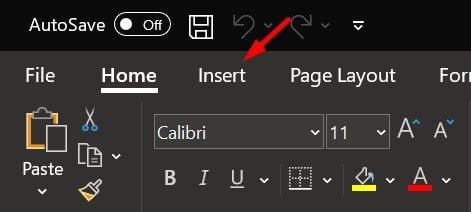
Step 2. Then, click on “Insert“. You can find it in the Menu bar right next to the Home option.
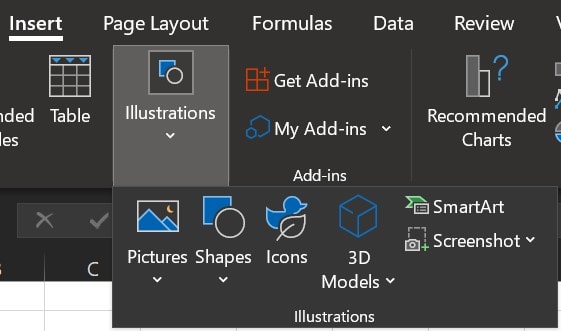
Step 3. Now, select “Shapes” from the ribbon. Sometimes, the Shapes option will be hidden under the “Illustrations” button.
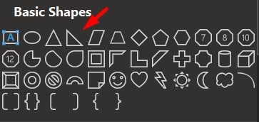
Step 4. Click on “Right Triangle” from the drop-down menu.
Step 5. Click anywhere on the sheet. It will display a right triangle.
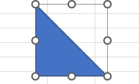
Step 6. You can also additionally rotate the figure as per your desire using the Format tab or using the rotate icon shown above the shape. Also, adjust the size according to your needs.
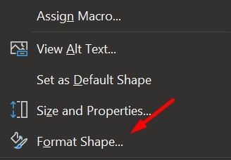
Step 7. After that, right-click on the Triangle Shape and select the “Format Shape” option.
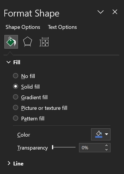
Step 8. Then, in the Format Shape Pane, do the following adjustments:
- First, select the Fill tab and toggle the Solid fill option.
- Then, choose a color for your Shape.
- Finally, close the pane.
Keep in mind that, you can make whatever changes you want using this pane. As a result, you will see the cell with a right triangle shaded as per your choice. You can now drag and place it on any cell you want.
Half-Fill Cells Diagonally using Fill Color
Instead of using the Shapes feature, you can also half-fill the cell directly with the Fill Color option. Let’s take a look at the steps involved.
Step 1. Start by launching Excel and opening a spreadsheet.
Step 2. After that, select a cell.
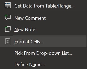
Step 3. Once it is highlighted, you can right-click on it.
Step 4. Now, choose “Format Cells” from the menu.
Doing so will launch a new dialogue box.
Step 6. In the Format Cells popup, search and click on the Fill tab.
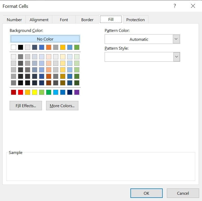
Step 7. Click on the “Fill Effects” button. It will open a box like this.
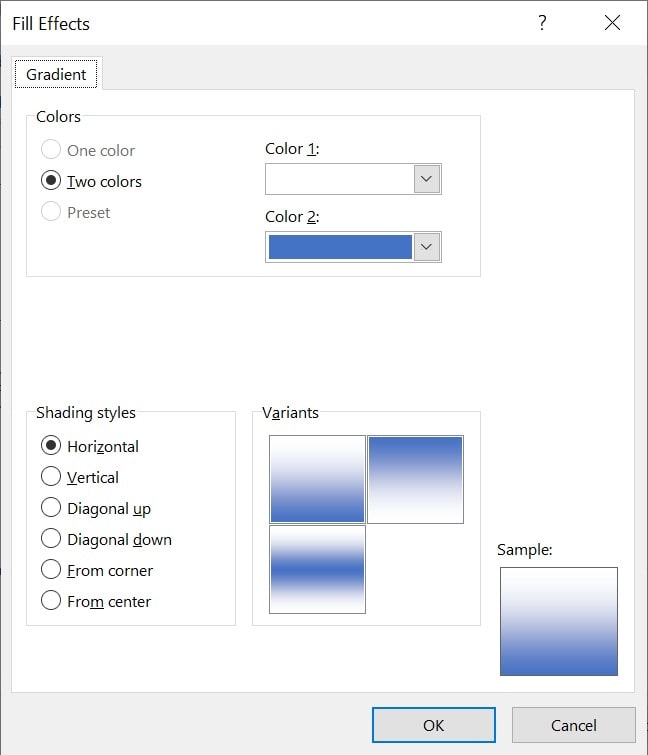
Step 8. Here, select the colors you want, since you want to half-shade a cell, we suggest choosing White as one of the colors. Also, change the shading style to diagonal.
Step 9. Now you have the option to shade the cell diagonally either up or down, select as per your preference.
Step 10. Once done with your selections, click on OK. The cell will be shaded.
Use Diagonal borders to half-fill
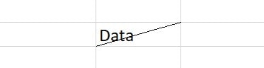
The final method that can help users half-fill a cell in Excel is undoubtedly the Diagonal borders feature that can automatically split the cell in half. The method adds a diagonal line to the cell that appears as if the cell is split in two. To proceed with this feature, follow the steps provided below:
Step 1. Select a cell. Once you have ensured the highlighted cell, go to the Format Tab (or click on the “Format” > “Format Cells…” option at the top ribbon). You can also right-click on the cell and choose the “Format Cells…” option.
Step 2. From the Format box, go to the Border tab and select the Diagonal line.
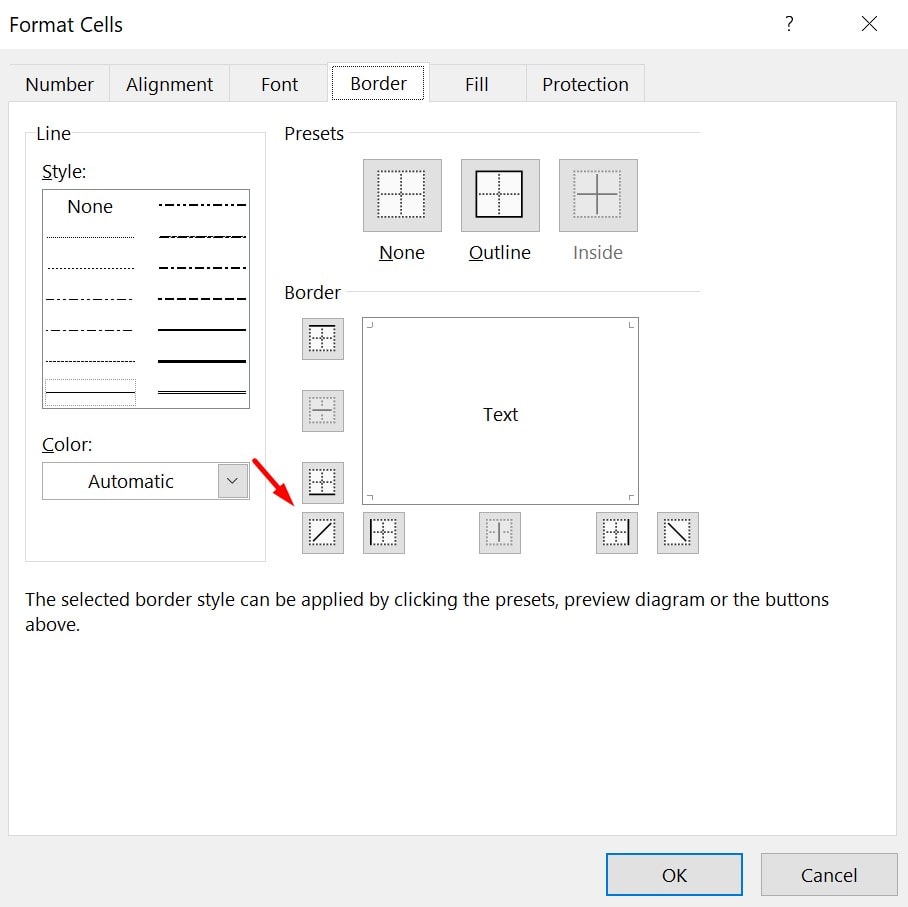
You can also customize the line itself, such as determining the thickness, style, or color. And then use the Fill tab to half-fill the cell if needed, following the steps mentioned in the above methods.
Step 3. Finally, click on OK to apply the border to the cell.
FAQ
Yes. Half-filling a cell is a process of making adjustments to the visual aspect while splitting cells splits the actual data contained in a cell.
Yes, you can. A triangle is the closest to a diagonal shape you can find. However, you can use any other shapes to be added to the cell. But, not sure if we can call it “half-fill” then.