Do you want to split the data of the cells into different columns? This might come in handy if you imported the data from somewhere else that is separated by a certain character, such as a comma or space.
Table of contents
Reasons to split cells in Excel
- Split data that was imported from another tool or software is separated by a unique character.
- Split text and numbers into different columns in your Excel sheet.
- Divide data into different columns to analyze them better.
- Split the first and second names from the full name column.
- To extract day, month, and year from a column that displays a date field.
2 Methods to split an Excel cell
Method 1. Using Delimiter to Split a cell in Excel
Delimiter is an Excel tool that is generally used to split a single cell into multiple ones. We can also use it to split cells. Here’s how:
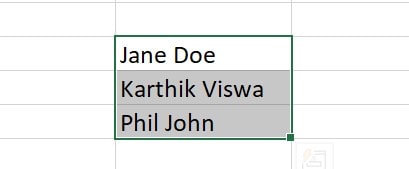
Step 1. Select the cell you want to split.
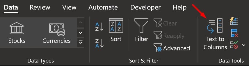
Step 2. Once you have ensured that the desired cell is highlighted, go to the top ribbon and click on the “Data” tab.
Step 3. Now, from the ribbon, choose the Text to Columns option.
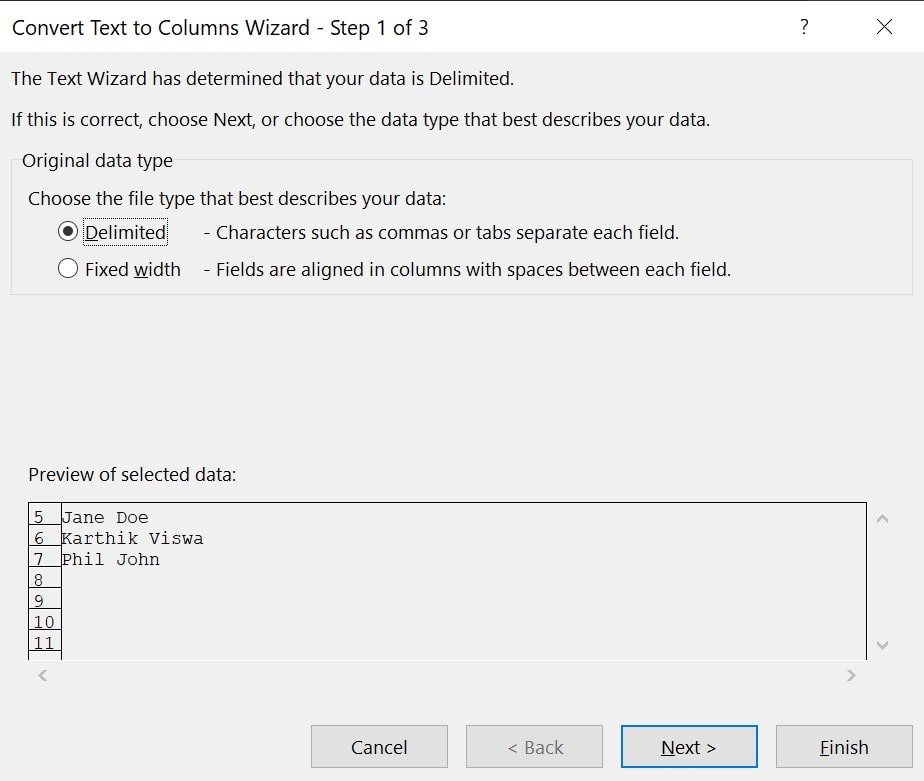
Step 4. This will launch the Convert Text to Columns Wizard.
Step 5. Here, select “Delimiter” as the file type. And proceed by clicking on the “Next” button.
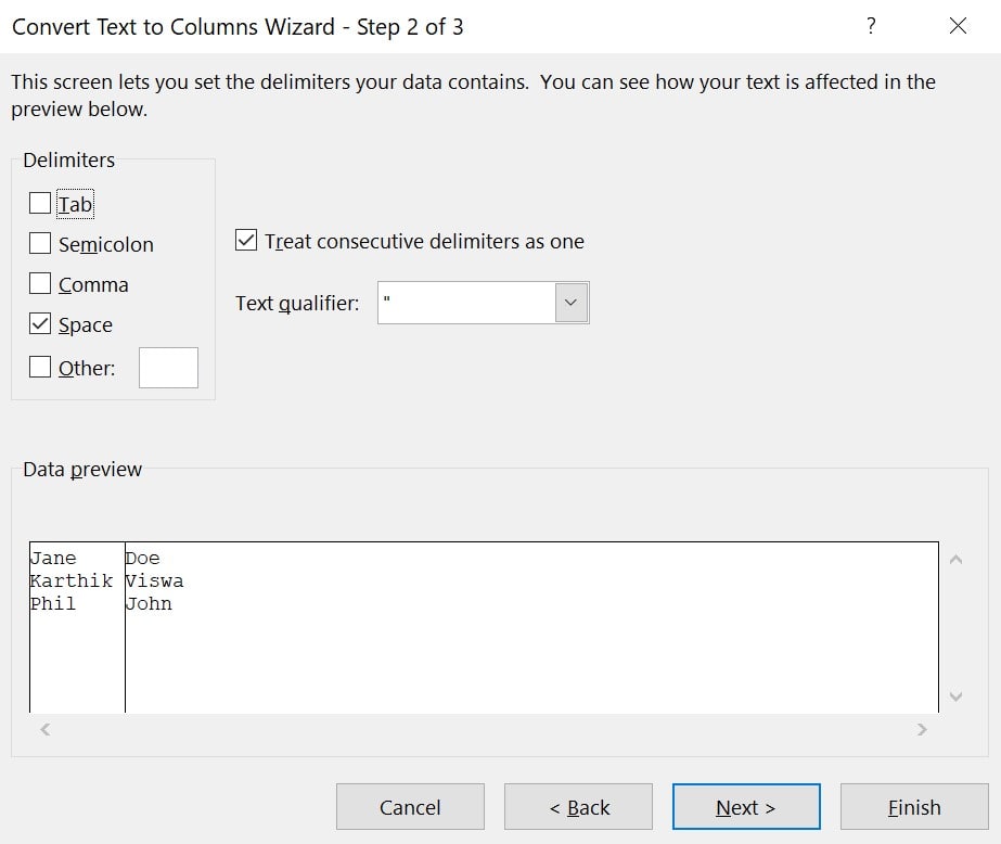
Step 6. Finally, click on the Next button after you have determined your delimiters to apply to the data. In this case, it is a “Space”.
Step 7. After that, go to the Format tab to decide how the data should appear. You can customize the following:
- General
- Text
- Date
- Do Not Import.
In most cases, you can leave it as it is. If your data is complex, you might have to configure it accordingly. You can check the “Data preview” below to see how your data looks after the changes.
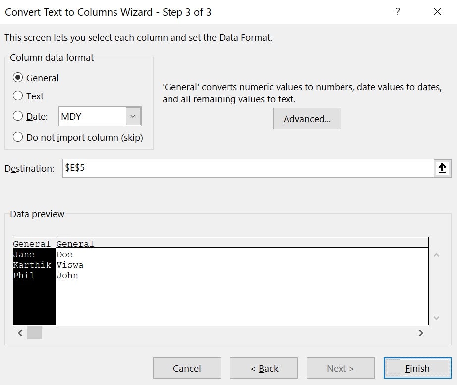
Step 8. Select the column to import the data to and finalize the destination for the cell. Once everything seems fine, click on “Finish”. It will split your data into two columns.

Method 2. Split the cell with the help of the Fixed Width Option
The next approach uses the Fixed Width option to split the cell. However, unlike the Delimiter method, these cells can be empty, and the method will still work. How? Let’s take a look:
Note: This will only work for cells with data that have a fixed number of characters and delimiters at a fixed place. You can still make this work if most of the data is like that. But you will have to manually edit it for the remaining.
Step 1. Launch the Excel Spreadsheet and select the cells with the data that you want to split.
Step 2. Then go to the Menu bar above and select the Data tab.
Step 3. After that, click on the Texts to Columns button.
Step 4. The Convert Text to Columns Wizard will launch. Here, select the Fixed Width Option and click Next.
Step 5. Now, select the point at which you want to split the cell. To do that, click on the scale shown under the Data preview section and drag it to where you want to split the data.
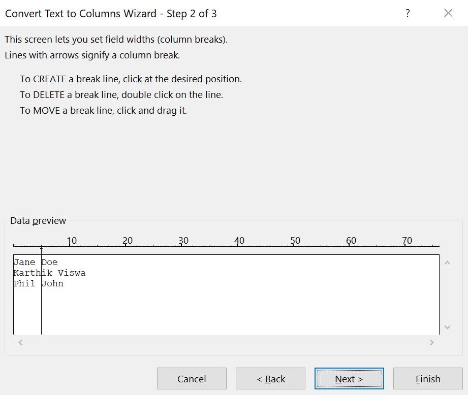
Step 6. Then, click on Next, and proceed to import the cell to a destination. When everything is set, click on the “Finish” button.