Create Drop-Down List in Excel: Basic, Dynamic, or Dependent

People are familiar with Excel. There is a whole generation of humans who grew up with the software. As such, millions of PC users know how to handle Excel. But the same people might have only scratched the surface as Excel is a treasure trove of features and functions.

The following article will explore how to create a drop-down list in Excel. Hence, those wanting to learn more about the topic can simply keep scrolling.

What is a drop-down list in Excel?

An Excel drop-down is a functionality that allows users to select data from a pre-defined set of values instead of typing them manually.

Hence, Excel drop-down list makes it easier to input data without having to manually type them into a cell, thus improving productivity. It is also a great data validation tool. Starting to use drop-down lists on your Excel sheets will significantly improve your productivity.

Benefits of an Excel drop-down list

• Data consistency: Drop-down lists are beneficial to make your data consistent across the column. You don’t have to worry about wrong values even if it’s a simple casing issue.
• Efficiency: Using drop-downs will allow you to input data much easier and faster, making your workflows seamless.
• Reduces data redundancy: By limiting the available options, the drop-downs can significantly reduce the chance of data redundancy in your Excel sheets.
• Easy analysis: You can analyze your data much better if you use Excel drop-down lists.

Today we are going to look at the possible methods you can follow to create a drop-down list in Excel within a few seconds.

Steps to create a drop-down list in Excel

Now, without further ado, let us dive right into the procedure of creating a drop-down list. We have documented a detailed set of steps to aid users in this endeavor. All you need to do is to follow these steps to successfully create a drop-down list.

Step 1. First, launch MS Excel on your PC and open a spreadsheet.

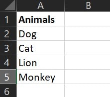
Step 2. Then proceed towards making entries that you want to appear in the list.

The ideal drop-down list has entries in a table. Thus, you would want to enter your data in an Excel table or convert your data later on by clicking Ctrl + T.

It is recommended to enter your data in a table because it can augment your drop-down list automatically when and if you add or remove data. Otherwise, you would have to manually update the drop-down list which is starting from scratch.

Step 3. Once you have made the necessary entries, it is time to create the list.

Thus, select the cells/column/row where you want the dropdown to appear and go to the Menu bar to select the Data tab.

You can select an entire row by clicking on the 1, 2, 3 items on the left, or the column by clicking on A, B, C, on the top.

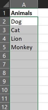
If your column has a header like this, you can simply hold down the Ctrl key and click on the header to exclude it from the selection.

Step 4. Now, click the Data tab and select Data Validation from the ribbon.

Step 5. After that, in the Settings tab, select List in the Allow section.

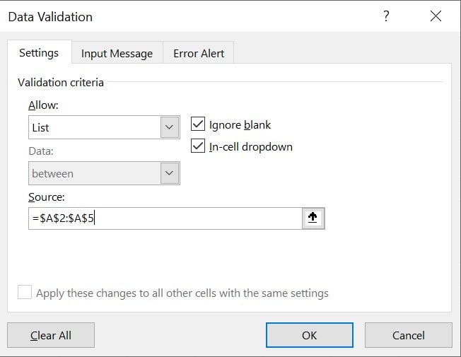
Step 6. Then go to Source input and finalize your list range by typing in the range. Or, you can simply use the button on the right side of the input box to select the area that contains the values you want to appear as the items in the drop-down list.

Step 7. Finally, make sure that the In-cell dropdown box is checked.

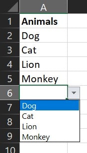
Step 8. Click the OK button. Now, when you click on any cell in that column, except the headline, you will see an option to select the items defined.

Now, those who want their list to showcase a message when the cell is selected, use the Input Message tab available in the Data Validation window. Same for the Error Message.

Using this feature, a user can display a message of up to 225 characters. Similarly, if you don’t want to show any messages, uncheck the boxes in the respective tabs.

Error Message

Drop-down lists exist to select data instead of creating entries. But users are still able to manually enter data in cells that are related to the drop-down list. However, if the entry is incorrect, an error alert is prone to show.

Although, this default error isn’t great at validating the type of acceptable data. Hence, users can manually improve this error alert up to their standards by using Data Validation. All the user has to do is ensure that the “Show error alert after invalid data is entered” box is ticked. After that, you can enter a new title and message for the error alert.

Input Message

Drop-down menus are great at preventing users from making incorrect data entries. Although the additional “Input Message” feature makes the overall operation more robust. While creating a drop-down list, users can add an input message by using the “Input Message” box in the Data Validation tab. It is an easy and secure way to improve user interaction and experience.

How to use the drop-down menu in an Excel table?

Now, we are aware that drop-down lists can be based on Excel tables for better functionality. However, if used in conjecture with another Excel table, the Drop-down list exudes magic. How?

When you add a drop-down list to the first cell of a table, Excel will automatically extend the drop-down to each new record. The steps are given below to demonstrate this process:

Step 1. First, open an Excel file and load a worksheet.

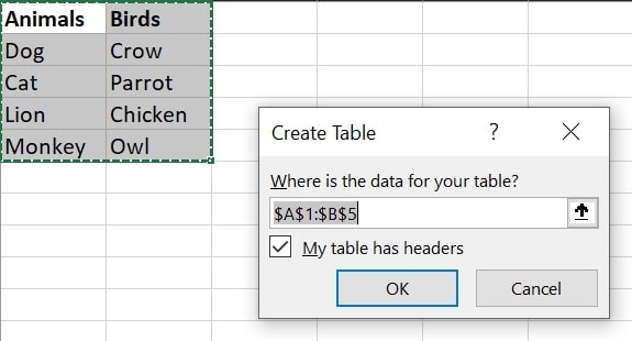
Step 2. After that, select the set of cells and transform them into a table by pressing Ctrl + T. Make sure to check the “My table has headers” option.

Step 3. Now, you need to make the first cell of the table a drop-down list. You can do that by following the method mentioned above. Make sure to choose all the cells in your table except the headline as the Source.

Step 4. Now, as you fill those cells, you will notice that the drop-down list items are getting updated. Click on the last table cell and press the Tab key on your keyboard to insert a new record into the table. As new records are being added, you will notice that your drop-down menu is also expanding.

Hence, it is that easy to use the drop-down menu in an Excel table.

Create a Dynamic Drop-down list

What we have created till now were normal drop-down lists, thus this time we will attempt a dynamic list where we can use a formula to automatically update the list if we add items to the end of the list.

Step 1. Select any cell you want to convert to a drop-down list.

Step 2. After that, go to the Data tab in the Menu bar and click on Data Validation.

Step 3. Now, choose List in the Allow section.

Step 4. It is time to enter the formula in the Source box. Enter the following formula in the box.

=OFFSET(Sheet2!$A$1,0,0,COUNTA(Sheet2!$A:$A),1)

It basically tells Excel to use the items in the first column of Sheet2 in the workbook as the values of the drop-down. You will have to create Sheet2 if it already doesn’t exist, or change it to Sheet1.

Step 5. Then click on Ok.

Now, whenever you enter any data into the first column in Sheet2, it will be automatically added to the drop-down list.

Create a Dependent Drop-down list

Lastly, we are going to touch upon the basics of a dependent drop-down list. The list is unique as there are two drop-down lists, but the second one is dependent on the first one.

For example, take a restaurant menu. Then list-1 can be the name of items, and list-2 can be the variant. When you select pizza from list-1, list-2 will show small, medium, large, or veg non-veg, etc.

Similarly, if you select Fried chicken in list-1, then list-2 will show grams, plates, or quantity. It means that although list-1 is visible, the choice can make list-2 change its contents. Hence, list 2 is dependent on list 1.

These are the steps to create a dependent drop-down list in Excel.

Step 1. Create the primary drop-down where you will input the data.

Step 2. Go to the Data tab.

Step 3. Click on Data Validation. It will open the Data Validation window.

Step 4. In the Settings Tab, as List under the Allow section.

Step 5. In the Source field, specify the ranges that you want as the primary drop-down items.

Step 6. Click on the OK button to create the first drop-down.

Step 7. Now, select the entire area with the data set.

Step 8. Go to Formulas Tab, and click on Create from Selection in the Defined Names group. There is also a shortcut to do this, Ctrl + Shift + F3. This will open the Create Names from the Selection window.

Step 9. In that window, check the Top row option and uncheck all the remaining.

Step 10. Click OK.

Step 11. Select the cell where you want the final drop-down to appear.

Step 12. Now again, go to Data > Data Validation.

Step 13. Select the List option as before in the Allow section.

Step 14. In the Source field, enter the following formula.

=INDIRECT(E6)

E6 is the cell where the main drop-down is located.

Also, if the main category name is multiple words, the formula should be:

=INDIRECT(SUBSTITUTE(E6,” “,”_”))

Step 15. Click OK.

That’s it. Now, try changing the first drop-down. You will notice that the second drop-down’s values are changing accordingly.

FAQ