Although decades old, Excel is still the topmost choice when it comes to spreadsheets and data entry. It is amongst the most powerful data visualization and analysis software available for both personal and professional use.
The software analyzes, stores, and tracks data with the help of a spreadsheet. As such, it is the first choice of marketers, analysts, and corporate workers. Since it is such a versatile tool, it is not impertinent that it has equal features.
These features are there to make the user’s life easier. But not every user is aware of these simple solutions. Hence, we have come up with the following article to help fellow Excel users. The article also includes tips and tricks to make your Excel journey seamless.
Table of contents
Pro Tips for a Smoother Excel experience

Given below are a few tips that can help you out when using Excel, do give them a try.
Transpose Rows into Columns
The transpose function is useful when you want to copy a set of data from rows to columns. It is also helpful when you copy data from another source. Such data will always get pasted vertically in rows. Thus, users tend to spend too much time, rearranging them into columns manually.
Follow these steps to transpose rows into columns in Excel:
Step 1. Select the range of data.
Step 2. Press Ctrl+C to copy it.
Step 3. And then go to the desired cell.
Step 4. Finally, right-click and select Paste and then transpose.
Text Wrap
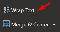
Re-sizing columns and rows is a necessity when it comes to data entry. Especially, when we want our presentation to look visually aesthetic. However, manually changing the shape of cells takes too much time. Thus, users are recommended to use the “Wrap Text” feature so that long strings of data can fit the entire cell without modification. This is usually located in the Home tab.
Add Multiple Rows or Columns
Adding a single row or column is pretty simple in Excel. However, users can also add multiple rows or columns at once. And it is done by using the Insert feature. Select multiple rows or columns before inserting to add the same number of rows or columns instead of 1.
Half-fill a cell diagonally
Sometimes there is a need to differentiate cells with different looks. Although there are various methods to half-fill a cell, there is a simple remedy for this. And that is to use the Border feature. Users should first go to the menu bar to look up the Fonts group. And then select Borders. But don’t stop there. Underneath you can choose More options which allows you to add a diagonal line to a cell.
Deleting Blank Cell
Sometimes, during data entry, a few cells are left blank. Thus, for the sake of uniformity and accuracy, one should mark all these cells and delete them. Although manually selecting these cells can take a long time. Hence, here the user is recommended to use the Filter feature.
Here’s how:
Step 1. First, select the desired column.
Step 2. Go to the Ribbon.
Step 3. Then click on Find & Select > Go To Special.
Step 4. Now, select the Blank option.
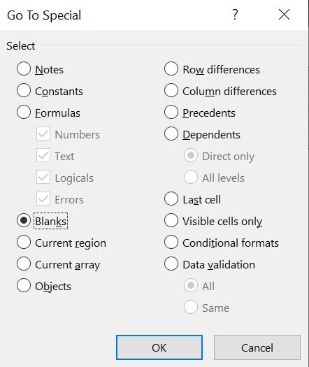
Step 5. Finally, click Delete on your keyboard to remove all the cells in one go.
Wild Card Vague Search
We all know that there is a search function that we can use by pressing Ctrl+F. But we can use two entries, Question Mark and Asterisk, to search the spreadsheet vaguely. It is used when the target result is unconfirmed. A Question Mark denotes a single character, and an Asterisk denotes more than one character.
Hide data from sight
It is also possible to hide data from plain sight. Just select the target cells, right-click, and choose Format cells. Then, on the number tab at the top, click on Category and choose Custom. Finally, type {;;;} and click on OK. Henceforth, the numbers will remain invisible, but you can still use them in formulas.
Multi-Select
Although dragging a mouse and selecting a dataset appears fast, there are better ways to do so. All you need to do is click on the first cell of the required dataset and press Ctrl+Shift and then press the down arrow to select all the data in the row below, up to select all the data above, the right arrow to select the data in the column on the right side and left for the left side. Furthermore, if you press Ctrl+Shift+End, it will select everything from the starting cell to the rightmost cell with data. While Ctrl+Shift+* might be faster, it tends to stop at blank cells, which can be an issue.
Insert Screenshot
Inserting a screenshot in Excel is pretty simple. Just go to the Insert tab at the Menu bar and select Screenshot. A drop-down menu will appear that will list the thumbnails of all the ongoing programs. Choose one, and the image will get imported.
Performing Quick analysis
The Quick Analysis feature lists some of the popular choices in Excel, such as formatting, charts, sparklines, formulas, etc. When in a hurry, select the set of data and run Quick Analysis and then choose what to do with the dataset.
Same data in multiple cells
Sometimes a user is required to enter the same data at different places. But manually entering the same data over and over is not only repetitive but also boring. Hence, be smart about it.
- First, select the set of cells.
- Then write the information on the last cell.
- Finally, press Ctrl+Enter.
- The same data will appear in all the selected cells.
Popular Shortcuts
Here is a list of some of the popular shortcuts that can make your life easier.
- Insert current date – Ctrl + ;
- Insert current time – Ctrl + Shift + :
- Change data format – Ctrl + Shift + #
- Font strike-through – Ctrl + 5
- Hide current column – Ctrl + 0
- Hide current row – Ctrl + 9
- Change Excel Workbook – Ctrl + F6
- Show all Formula – Ctrl + `
- Quick Scroll – Ctrl + PageUp/PageDown
- Edit current cell – F2
- Right-click prompt – Shift + F10
Use “&” to combine cells
Sometimes data is recorded under different multiple titles or headings. For example, a name could be recorded as a first name and a last name. But what if you require a single cell for the name? All you need to do is combine data under the First and Last name rows. This can be done by using the & sign in the formula. Suppose you want to join A2 and B2 then the formula would be:
=A2&” “&B2Add Hyperlinks
Adding Hyperlinks is pretty simple in Excel just copy and paste it. But in case that doesn’t work, or you need to highlight a particular word as a hyperlink, you should use the Ctrl + K command.
The Format Painter function
As you may know, Excel is a feature-rich program that is equally good at mathematical operations. However, formatting cells manually is often a chore. If you have to apply the same formatting over and over to each and every cell on a different worksheet, then use the Format Painter feature.