Excel is an excellent tool for data integration. It is not only perfect for recording various data sets, but it is also equally capable of using the same data for mathematical operations.
The program uses formulas to execute such operations. Hence, these formulas can be valuable if unique or if someone doesn’t want their data to get stolen. That’s why Excel allows users to input data without displaying the formulas if they want to. But how?
The following article will discuss the various methods to hide/display formulas in Excel, either for the whole sheet or for custom cells.
Table of contents
Why should you hide Formulas?
- To simplify the Excel sheet.
- Protect some confidential information.
- Prevent the formulas from being accidentally changed.
- Prevent others from copying your formulas to their own sheets.
Methods to hide Formulas in Excel
Given here are the common methods to hide formulas in Excel, let’s take a look!
Method 1. Using the Formula Ribbon
The very first method we can incorporate is via using the formula ribbon. Here’s how:
Step 1. Load a worksheet and select a cell with a formula to hide.
Step 2. Now, click on the Formula icon/tab.
Step 3. After that, click on the “Show Formulas” button.
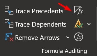
Now, the formulas will stop displaying. Use the same process to display the formula once again.
Method 2. Manually hide Formula from one cell at a time
You can also hide the formula for a single/custom cell without relying on the Show Formula button. And that is to use the keyboard shortcut of Ctrl + `.
Methods 3. Preventing the Formula from displaying in the Formula Bar
The following method will ensure that the formulas won’t get displayed even in the formula bar. Thus, virtually making the cell unable to be edited. The steps are:
Step 1. First, launch MS Excel and load a worksheet.
Step 2. Either select a set of cells, adjoining cells, a single cell, or the entire worksheet.
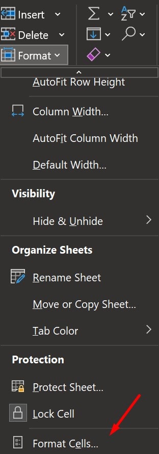
Step 3. Now, go to the Menu bar and click on the “Format” button.
Step 4. Then, select the “Format Cells” option.
Step 5. Navigate to the “Protection” tab from the dialogue box and check the “Hidden” checkbox.
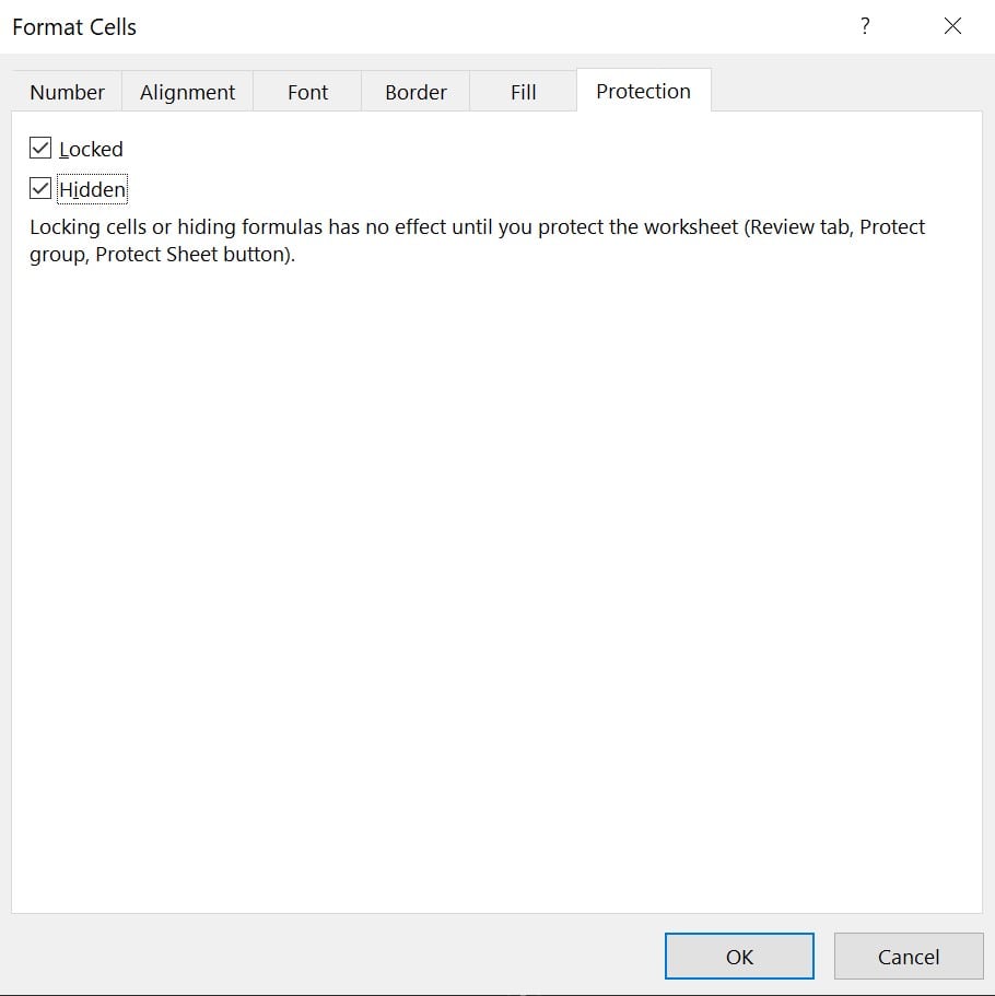
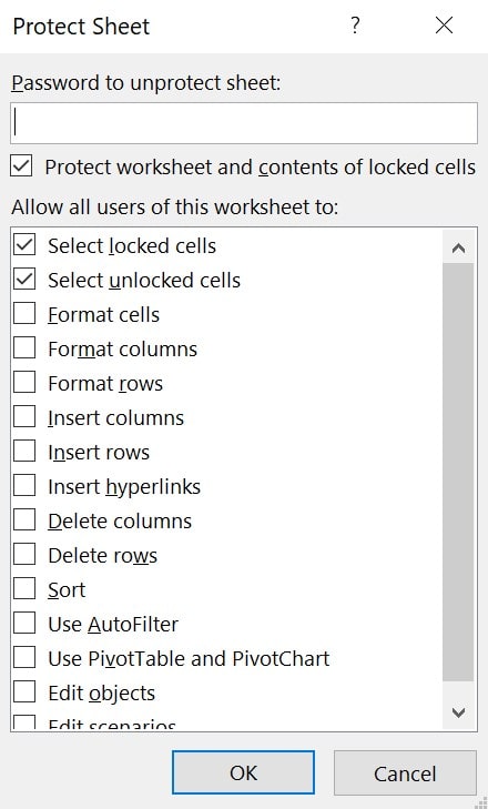
Step 6. As you can read from there itself, this will not have any effect unless you protect the sheet. To protect the sheet, go to the “Review” tab.
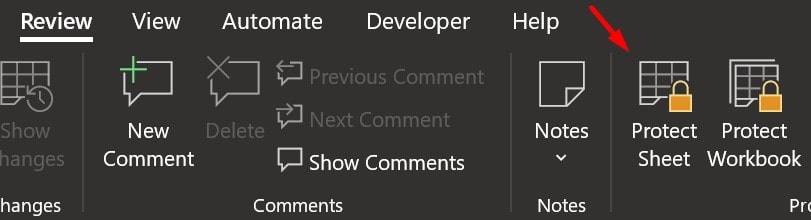
Step 7. Then “Protect Sheet“. Then fill out the necessary details such as the password.
Hide all formulas and Protect the worksheet
Now, we will look at a process where users can not only protect their entire worksheet but also hide the corresponding formula. These methods are:
Method 1
The following method will not only ensure other users from making any changes to your datasheet but also prevent them from viewing formulas. Even if the user clicks on a cell, he will only see a blank entry.
Step 1. First, start the Excel program and load a worksheet. Remember that the sheet must be unprotected for this method to work.
Step 2. Now, visit the Menu bar and locate the “Review” tab.
Step 3. Click it and find the “Protect sheet” button. Press it, and fill out the necessary details. Now your sheet is protected.
Step 4. After that, manually select the cells whose formulas you want to remain hidden and right-click.
Step 5. Then click on “Format” > “Format Cells” options and navigate to the “Protection” tab.
Step 6. Since you have already protected the worksheet, you will find the Locked toggle engaged. All you have to do is toggle the Hidden box.
Always remember that the Hidden box toggle won’t work if your sheet is unprotected.
Method 2
There is a different method for the same solution, which we will discuss now. But first, you should comprehend that when you enter a formula in any cell, users can see it via two different methods –
- Either by double-clicking on the cells and getting to the edit mode.
- Or by clicking on the cell and viewing the formula from the Formula bar.
Hence, this method will ensure that both the above-mentioned approaches don’t work. And here’s how:
- Manually select the cells you want to hide.
- Now, on the Menu bar, go to the Home tab.
- Then, in the Number group, click on the dialog box (the downward arrow in the bottom right corner).
- After that, choose Format cells and click on the Protection tab.
- Here, toggle the Hidden option, and select OK.
- Now visit the Review tab and go to the Protect Sheet.
- You can now enter a password to safeguard your worksheet.
- Now that your entire worksheet is protected, your cells will remain hidden.
Remember that since that worksheet is protected, you also can’t edit any cells. Thus, for those who want to hide a formula and still want to make other changes to a worksheet, then follow the steps below.
Hide only Formulas and allow other changes to the worksheet
This method can aid those users who want to hide their data and still want to make other changes to the worksheet can follow the steps below:
Phase 1. Disable worksheet lock
First, we need to disable the locked worksheet.
Step 1. To do so, users need to select the entire worksheet. Hence, press Ctrl + A.
Step 2. Now open the Formal Cell dialog by pressing Ctrl + 1.
Step 3. Go to the Protection option and ensure that the Locked box is unchecked.
Step 4. Then click OK.
Phase 2. Hide formulas
Since the sheet is now unlocked, we need to select the cells and hide the formulas manually.
Step 1. Thus, select the required cells.
Step 2. Then go to the Home tab and click on the Find & Select button.
Step 3. After that, choose Go To Special.
Step 4. And then, check the toggle Formula box to select only cells with formulas.
Step 5. Once you have selected the required cells, open the Format cell dialog box, either by right-clicking or by pressing Ctrl + 1.
Step 6. Now approach the Protection tab and ensure that both Locked and Hidden boxes are checked.
Step 7. Finally, click on OK, and to protect your worksheet, go to the Review ribbon and choose the Protect Sheet option.
Since the sheet is now protected, the cells are locked and hidden. And since we applied them specifically to those cells containing formulas.
The user can now edit the worksheet and at the same time ensure the formals remain hidden, this method is by far the most versatile one. However, when hiding new cells, one has to unlock the whole sheet and follow the steps prescribed here once again.
Otherwise, the user can simply keep on editing those cells without any formulas or add new values to the worksheet.