Freezing rows in Excel is an excellent way to make the important rows stick to the top of the sheet as you scroll down. This way, you will not have to scroll all the way up whenever you have to cross-check some facts.
This can be especially useful if you have a heading row. Once you make the row freeze, it will follow as you scroll.
Table of contents

Freeze Panes to Lock rows and columns
The following segment will highlight steps necessary to freeze panes in Excel running on a Windows device.
Freeze Rows
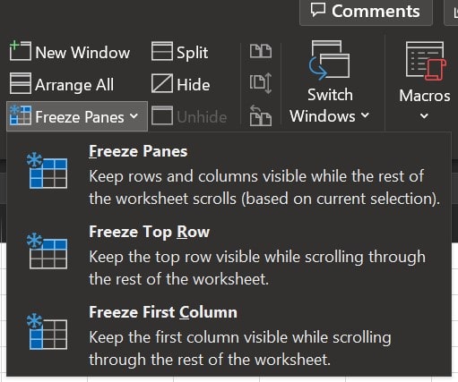
We can freeze rows in Excel in just a few clicks. All the user has to do is click on View tab and then select Freeze Panes. Here the user will have more than one option which we have explored in the upcoming sections.
The necessary steps to freeze rows are as follows:
Freeze Top Row
When the user has to freeze only the top row of a sheet, he can do the following:
- Open an Excel sheet.
- Go to menu bar and click on View tab.
- Then select Freeze Panes.
- And finally, click on Freeze Top Row.
Freeze multiple rows
Similarly, users can always utilize the Freeze Panes section to lock multiple rows at once.
- Click on a row or cell that is right below the last row you want locked.
- For example, if you want to freeze rows 1 to 5 then click on Row 6 or cell A6.
- Similarly, if you want to freeze the top 3 rows then click in the fourth row or cell A4.
- Again, go to the menu bar and click on the View tab.
- After that, click on Freeze Panes, and choose Freeze Panes from the drop-down menu.
Freeze Columns
The process of locking columns is exactly similar to rows, which we will examine in the following sections.
Freeze The First Column
In order to freeze the first column, do the following:
- Open an Excel sheet.
- Then, click on the View tab in the menu bar.
- After that, click on Freeze Panes and select Freeze First Column.
Freeze multiple Column
Those who want to freeze more than one column, should follow these steps:
- Select the column right next to the last column you want locked.
- After that, go to the menu bar, click on View tab and select Freeze Panes.
Freezing both rows and columns
If you want to freeze both rows and columns together, then it is a simple process as the user should:
- First, open an Excel sheet.
- Then, click on a row just below the last row you want to lock and a column right next to the column you want locked.
- For example if you want to lock rows 1 to 3 and column A to D then you should click on the row 4 in column E or cell E4.
- After that, go to the menu bar, click on View tab and select Freeze Panes to lock the designated rows and columns.
Those using Excel 2013, or 2016 versions can also use the same steps mentioned above.
Unlock Rows and Columns
Unfreezing or unlocking rows and columns are even easier, and just one click away. All the user has to do is go to the menu bar, then go to the View tab, and then select Freeze Panes. Finally, click on Unfreeze Panes to unlock the rows and columns.
Troubleshoot Freeze Panes not working
If by some chance your Freeze Panes button is not working, disabled or greyed out, it’s most likely due to the following reasons:
- You are editing the cell in question, i.e. you are either working on it like entering or editing a data or entering any formula. Just click on enter to cease cell editing and try again.
- You are working on a protected worksheet. Hence, you need to remove the protection before you can freeze rows or columns.